So why do we need to initialize weights in deep learning?

Published on: May 22, 2024

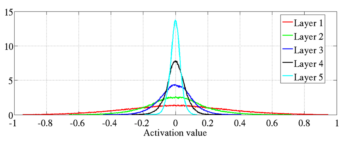
Here's a visualization of how mean activation and gradient values differ with and without initialization. These experiments were performed in the paper that introduced "Xavier initialization." The researchers used a 5-hidden-layer network for their analysis.

Fig: 1. Activation values with standard initialization 2. Gradient values with standarad initialization : Source Xavier initilization

Fig: 2. Activation values with xavier initialization 2. Gradient values with xavier initialization : Source Xavier initilization

Without initialization (standard initialization), activation and gradient values tend to vanish. This is evident in the gradient value histogram, where backpropagation leads to vanishing values as we move from layer 5 to layer 1. The figure above clearly demonstrates the need for initialization, as seen in the second picture. But why does initialization lead to such consistency? Let's explore this next.

y_l = W_l * x_l + b_l

In the following equation, bold letters are used to represent vectors. To define every term in the equation:

$W_{l}$ is the weight matrix of size $d_{l} - to - n_{l}$ from layer l-1 to l.
$x_{l}$ is the output of l-1 layer that was passed through activation function f(.). It is a $n_{l} - by - 1$ vector.
$b_{l}$ represents biases of layer l.
$y_{l}$ is the output of the layer l before it is passed to an activation function.

Some assumptions have to be made to move further:

Elements of $W_{l}$ are independent to each other and share the same distribution.
Elements of $x_{l}$ are independent to each other and share the same distribution.
Both $W_{l}$ and $x_{l}$ are independent to each other.

W_{l} x_{l} = [\begin{matrix} \sum_{i = 1}^{n_{l}} w_{1, i} x_{i} \\ \sum_{i = 1}^{n_{l}} w_{2, i} x_{i} \\ . \\ . \\ \sum_{k = 1}^{n_{l}} w_{d, i} x_{i} \end{matrix}]

If we take variance of this expression than we get a diagonal matrix, because of the independence of the variables. Variance of the right handside is eqal to the trace of the covariance of the left handside (need to see why).

Var [W_{l} x_{l}] = Tr [\begin{matrix} var [\sum_{i = 1}^{n_{l}} w_{1, i} x_{i}] & 0 & . & 0 \\ 0 & var [\sum_{i = 1}^{n_{l}} w_{2, i} x_{i}] & . & 0 \\ . & . & . & . \\ 0 & 0 & 0 & var [\sum_{i = 1}^{n_{l}} w_{d, i} x_{i}] \end{matrix}]

= \sum_{j = 1}^{d_{l}} v a r [\sum_{k = 1}^{n_{l}} W_{j, k} * x_{k}]

Because the variables are independent to each other variance of sum is sum of variance,

v a r [X + Y] = v a r [X] + v a r [Y]

v a r [W_{l} x_{l}] = \sum_{j = 1}^{d_{l}} \sum_{k = 1}^{n_{l}} v a r (W_{l} x_{l}) = d_{l} * n_{l} * v a r (W_{l} x_{l})

Further, simplifying it we get,

v a r [y_{l}] = d_{l} * v a r (y_{l})

Relation between variance and expectation is given by,

v a r (X) = E [X^{2}] - E [X]^{2}

So,

v a r [y_{l}] = n_{l} * (E [{w_{l}}^{2}] * E [{x_{l}}^{2}] - E [w_{l}]^{2} * E [x_{l}]^{2}])

If we choose the distribution of w_l such that its mean is zero, then we can write,

v a r [y_{l}] = n_{l} * v a r [w_{l}] * E [{x_{l}}^{2}]

Note that we aren't making any assumptions about the mean of x_l so,

E [{x_{l}}^{2}] \neq v a r [x_{l}]

Two of the most popular initilization techniques are kaiming and xavier initialization. Xavier doesn't take activation into account while kaiming does. Let's move forward with kaiming initilization. Lets assume activation used in the previous layer is ReLU activation, which is given by,

R e L U (x) = \{\begin{cases} x & i f x \geq 0 \\ 0 & i f x < 0 \end{cases}

E [{x_{l}}^{2}] = E [m a x {(0, y_{l - 1})}^{2}] = \frac{1}{2} E [{y_{l - 1}}^{2}] = \frac{1}{2} var [x_{l - 1}]

How did we get that (1/2)? Here, we assume that

w_{l - 1}

has zero mean and symmetric distribution around 0 and

b_{l - 1} = 0

. So,

y_{l - 1}

has zero mean and has a symmetric distribution around zero. So, probability of

y_{l - 1}

>0 is 1/2.

var [y_{l}] = n_{l} var [w_{l}] * \frac{1}{2} var [y_{l - 1}]

We can establish a recursive realtion from the above equation which is given by

var [y_{L}] = var [y_{1}] (\prod_{l = 2}^{L} \frac{1}{2} n_{l} var [w_{l}])

This equation explains everything. For very deep neural networks (large L), if the term in brackets is less than 1, the variance of the activations in the final layer tends to shrink dramatically. Conversely, if the term is greater than 1, the variance can explode. This highlights why the ideal value within the brackets is 1. It helps maintain a balanced flow of gradients throughout the network, preventing both vanishing and exploding gradients during training.

\forall l, \frac{1}{2} n_{l} var [w_{l}] = 1

An intersting observation is that the variance of first layer does not make much of a difference.

References

How to initialize deep neural networks? Xavier and Kaiming initialization | Here
Delving Deep into Rectifiers: Surpassing Human-Level Performance on ImageNet Classification